
검색결과 리스트
글
Part I: Applied Math and Machine Learning Basics
5. Machine Learning Basics
여기서 부터는 전개 방식을 변경해 영어 원문과 요약으로 전개해나갈 예정입니다.
5.7 Supervised Learning Algorithms
Recall from Sec. 5.1.3 that supervised learning algorithms are, roughly speaking, learning algorithms that learn to associate some input with some output, given a training set of examples of inputs \(x\) and outputs \(y\). In many cases the outputs \(y\) may be difficult to collect automatically and must be provided by a human “supervisor,” but the term still applies even when the training set targets were collected automatically.
Supervised learning은 입력 \(x\)와 출력 \(y\)에 대해 입력과 출력을 연관시키는 것을 학습한다.
대부분 \(y\)를 자동으로 생성하기 힘들어서 “supervisor”가 제공해야 하지만, 자동으로 생성된 경우도 여기에 해당함.
5.7.1 Probabilistic Supervised Learning
Most supervised learning algorithms in this book are based on estimating a probability distribution \(p (y\ |\ x)\). We can do this simply by using maximum likelihood estimation to find the best parameter vector \(\theta\) for a parametric family of distributions \(p (y\ |x;\theta)\).
이 책의 supervised learning 알고리즘은 확률 분포 \(p (y\ |\ x)\)를 추정하는 것을 기본으로 하고, 분포의 parametric family \(p (y\ |x;\theta)\) 의 최적의 \(\theta\)를 maximum likelihood estimation을 통해 구할 수 있다.
We have already seen that linear regression corresponds to the family
앞에서 linear regression 예를 들어 maximum likelihood estimation가 normal distribution인 경우,
\[p\ (y|\ x;\theta)=\mathcal{N}(y;\theta^{\mathrm{T}}x,\ I)\tag{5.80}\]
We can generalize linear regression to the classification scenario by defining a different family of probability distributions. If we have two classes, class 0 and class 1, then we need only specify the probability of one of these classes. The probability of class 1 determines the probability of class 0, because these two values must add up to 1.
이 family를 여러개 정의해서 linear regression을 classification으로 일반화 할 수 있다(예를 들어 \(\mathcal{N}(y=0;\theta^{\mathrm{T}}x,\ I)\), \(\mathcal{N}(y=1;\theta^{\mathrm{T}}x,\ I)\)...).
그런데 class가 0과 1만 있는 경우는 하나만 정의하면 된다. 왜냐하면 0일 확률과 1일 확률을 더하면 1이 되어야 하기 때문이다.
The normal distribution over real-valued numbers that we used for linear regression is parametrized in terms of a mean. Any value we supply for this mean is valid. A distribution over a binary variable is slightly more complicated, because its mean must always be between 0 and 1. One way to solve this problem is to use the logistic sigmoid function to squash the output of the linear function into the interval (0, 1) and interpret that value as a probability: This approach is known as logistic regression (a somewhat strange name since we use the model for classification rather than regression).
위의 normal distribution에서 parametrized되는 것은 평균이다. binary 변수(0과 1의 값만 가짐)의 경우 distribution이 좀더 복잡한다, 평균이 항상 0과 1사이에 있어야 하기 때문이다.
이를 해결하기 위해 logistic sigmoid function을 사용하여 선형 함수의 출력을 0과 1사이의 값으로 변환해 주는 것이다.
\[p\ (y=1\ |\ x;\theta)=\sigma(\theta^{\mathrm{T}}x)\tag{5.81}\]
This approach is known as logistic regression (a somewhat strange name since we use the model for classification rather than regression).
이런 접근법을 logistic regression 이라고 한다.
In the case of linear regression, we were able to find the optimal weights by solving the normal equations. Logistic regression is somewhat more difficult. There is no closed-form solution for its optimal weights. Instead, we must search for them by maximizing the log-likelihood. We can do this by minimizing the negative log-likelihood (NLL) using gradient descentP>
Linear regression은 normal equation \(\left(w=\left( X^{\top}X \right)^{-1} X^{\top}y\right)\) 을 풀어서 쉽게 weight를 찾을 수 있었는데, logistic regression의 경우는 쉽지 않다. 여기서는 log-likelihood를 maximize하기 위해 gradient descent를 사용해 negative log-likelihood를 minimize한다.
This same strategy can be applied to essentially any supervised learning problem, by writing down a parametric family of conditional probability distributions over the right kind of input and output variables.
이 방법은 모든 supervised learning 문제에 적용 가능하다(input과 output을 올바로 지정해야 함).
5.7.2 Support Vector Machines
One of the most influential approaches to supervised learning is the support vector machine ( Boser et al. , 1992 ; Cortes and Vapnik , 1995 ). This model is similar to logistic regression in that it is driven by a linear function \(w^{\mathrm{T}}x+b\). Unlike logistic regression, the support vector machine does not provide probabilities, but only outputs a class identity. The SVM predicts that the positive class is present when \(w^{\top}x+b\) is positive. Likewise, it predicts that the negative class is present when \(w^{\top}x+b\) is negative.
Support vector machine(SVM)은 Supervised learning의 대표적인 접근법 중 하나다.
선형 함수 \(w^{\top}x+b\)에 의해 구동된다는 점에서 logistic regression과 유사하지만, 확률 대신 class ID만 출력한다. \(w^{\top}x+b\)가 양수일 때와 음수일 때로 클래스를 구분(+1, -1)한다.
One key innovation associated with support vector machines is the kernel trick. The kernel trick consists of observing that many machine learning algorithms can be written exclusively in terms of dot products between examples. For example, it can be shown that the linear function used by the support vector machine can be
SVM의 Key innovation(혁신)은 kernel trick이다. Kernel trick은 많은 Machine learning 알고리즘이 example 간의 dot product로 쓰일 수 있다는 데서 출발한다. 예를 들어, linear function에 SVM을 사용하면 다음과 같다:
\[w^{\top}x+b=b+\displaystyle \sum_{i=1}^{m}\alpha_i x^{\top}x(i)\tag{5.82}\]
-------------------------식 (SVM)관련 추가 설명-------------------------------------------------------
Decision boundary가 선형이고 아래 그림처럼 Margin은 \(\frac{2}{{\sqrt {{{\bf{w}}^T}{\bf{w}}} }}\)가 된다.
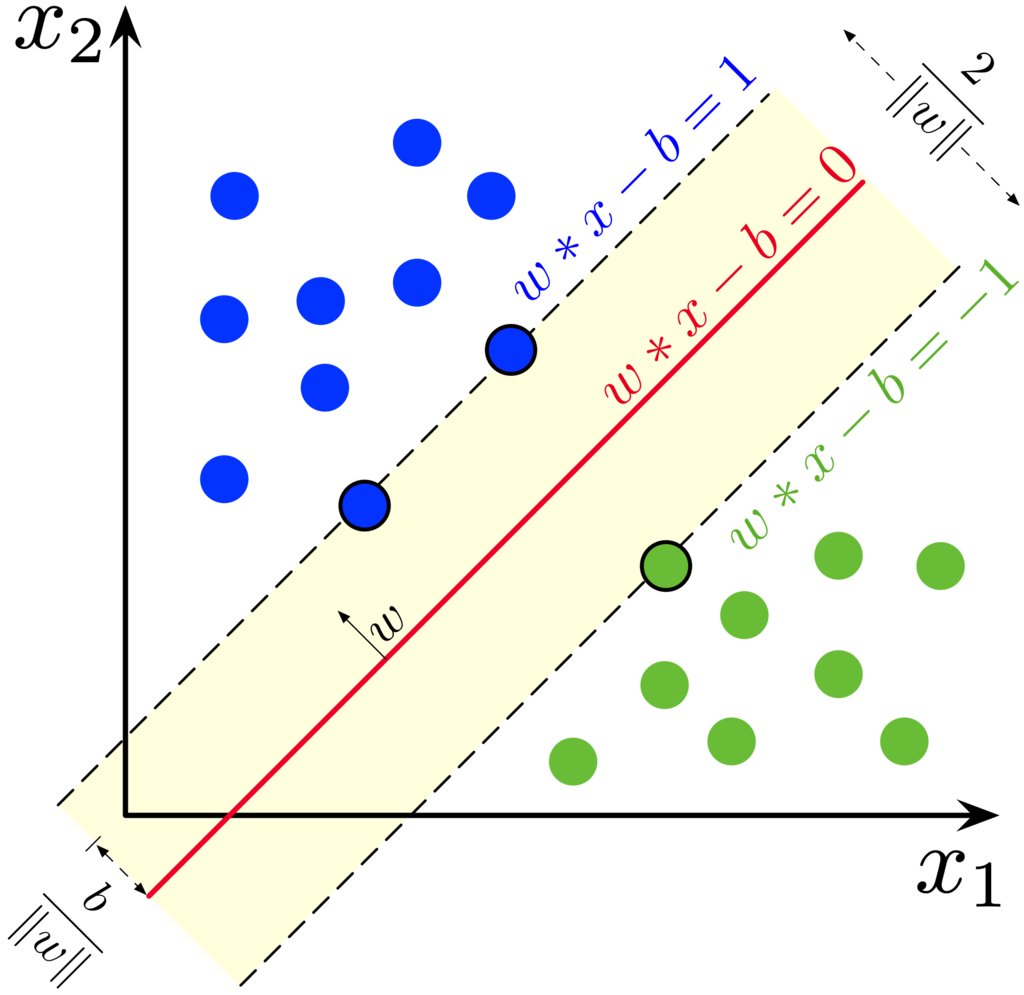
이미지 출처 : http://en.wikipedia.org/wiki/Support_vector_machine
Margin \(\frac{2}{{\sqrt {{{\bf{w}}^T}{\bf{w}}} }}\)을 최대화 하려면 \({w^ \top }w\)를 최소화 해야하며, \({y^{(i)}}({w^ \top }x + b) \ge 1\)을 만족해야 하므로, Constrained Optimization이다. Lagrange Multipliers를 이용해 unconstrained optimization로 만들어 주면
\[{\cal L}\left( {w,b,\alpha } \right) = \frac{1}{2}{w^ \top }w - \sum\limits_i^m {{\alpha ^{(i)}}{y^{(i)}}\left[ {({w^ \top }x + b) - 1} \right]} ,\quad {\alpha ^{(i)}} > 0\]
위 식에서 \(w\)에 대해 미분하면
\[\frac{\partial }{{\partial w}}{\cal L}\left( {w,b,\alpha } \right) = w - \sum\limits_i^m {{\alpha ^{(i)}}{y^{(i)}}} = 0\]
위 식에서 \(w = \sum\limits_i^m {{\alpha ^{(i)}}{y^{(i)}}} \)를 얻을 수 있고, 여기서 \(y^{(i)}\)가 식 5.82의 \(x^{(i)}\)에 해당한다.
------------------------------------------------------------------------------------------------
where \(x^{(i)}\) is a training example and α is a vector of coefficients. Rewriting the learning algorithm this way allows us to replace \(x\) by the output of a given feature function \(\phi(x)\) and the dot product with a function \(k(x,\ x^{(i)})=\phi(x)\cdot\phi(x^{(i)})\) called a kernel. The · operator represents an inner product analogous to \(\phi(x)^{\top}\phi(x^{(i)})\). For some feature spaces, we may not use literally the vector inner product. In some infinite dimensional spaces, we need to use other kinds of inner products, for example, inner products based on integration rather than summation. A complete development of these kinds of inner products is beyond the scope of this book.
여기서 \(x\)를 feature function \(\phi(x)\)로 대체 할 수 있고, 내적 함수 \(k(x,\ x^{(i)})=\phi(x)\cdot\phi(x^{(i)})\)를 kernel이라고 한다. (일부 내적을 할 수 없는 feature spaces도 있고, 적분을 해야하는 경우도 있지만 여기서는 다루지 않음)
After replacing dot products with kernel evaluations, we can make predictions using the function
\(f(x)=b+\sum\limits_i \alpha_{i}k(x,x^{(i)})\ \tag{5.83}\)
This function is nonlinear with respect to \(x\), but the relationship between \(\phi(x)\) and \(f(x)\) is linear. Also, the relationship between \(\alpha\) and \(f(x)\) is linear. The kernel-based function is exactly equivalent to preprocessing the data by applying \(\phi(x)\) to all inputs, then learning a linear model in the new transformed space.
\(\phi\)는 비선형 함수이다. (이 함수와 \(x\)도 비선형) Kernel 기반 함수는 모든 입력에 \(\phi(x)\)를 적용한 뒤 변환된 새 공간에서 선형 모델을 학습하는 것과 정확히 같다.
The kernel trick is powerful for two reasons. First, it allows us to learn models that are nonlinear as a function of \(x\) using convex optimization techniques that are guaranteed to converge efficiently. This is possible because we consider \(\phi\) fixed and optimize only \(\alpha\), i.e., the optimization algorithm can view the decision function as being linear in a different space. Second, the kernel function \(k\) often admits an implementation that is significantly more computational efficient than naively constructing two \(\phi(x)\) vectors and explicitly taking their dot product.
Kernel Trick의 두가지 장점:
① \(\phi\)가 고정되고, \(\alpha\)만 최적화 된다고 생각하기 때문에 convex 최적화 이다.
② Kernel 함수 \(k\)를 사용하는 것이 종종 순수하게 두 \(\phi(x)\)를 구하고 dot product한것 보다 계산적으로 효율적이다.
In some cases, \(\phi(x)\) can even be infinite dimensional, which would result in an infinite computational cost for the naive, explicit approach. In many cases, \(k(x,\ x')\) is a nonlinear, tractable function of \(x\) even when \(\phi(x)\) is intractable. an example of an infinite-dimensional feature space with a tractable kernel, we construct a feature mapping \(\phi(x)\) over the non-negative integers \(x\). Suppose that this mapping returns a vector containing \(x\) ones followed by infinitely many zeros. We can write a kernel function \(k(x,\ x^{(i)}) = \min(x,\ x^{(i)})\) that is exactly equivalent to the corresponding infinite-dimensional dot product.
\(\phi(x)\)가 계산이 어렵더라도, \(k(x,\ x')\)는 대부분 계산하기 쉬운 함수이다. 계산하기 쉬운 무한 차원의 feature space의 한 예로, 음수가 아닌 정수 \(x\)를 \(\phi(x)\)를 통해 매핑한다고 생각해 보면, \(\phi(x)\)는 1과 무수히 많은 0을 가지는 무한 차원의 벡터를 반환한다고 가정했을 때, 이를 내적 하는 kernel 함수는 \(k(x,\ x^{(i)}) = \min(x,\ x^{(i)})\)로 간단하게 구할 수 있다.
The most commonly used kernel is the Gaussian kernel
가장 일반적으로 사용되는 kerenl은 Gaussian kernel이다.
\[k(u,\ v)=\mathcal{N}(u-v;0,\ \sigma^{2}I)\tag{5.84}\]
where \(\mathcal{N}(x;\mu,\ \Sigma)\) is the standard normal density. This kernel is also known as the radial basis function (RBF) kernel, because its value decreases along lines in \(v\) space radiating outward from \(u\). The Gaussian kernel corresponds to a dot product in an infinite-dimensional space, but the derivation of this space is less straightforward than in our example of the \( \min\) kernel over the integers.
\(\mathcal{N}(x;\mu,\ \Sigma)\): Standard normal density.
이 kernel은 Radial Basis Function(RBF)라고도 한다. Gaussian kernel은 무한 차원 공간에서의 내적에 해당하지만, 공간의 전개는 min kernel의 경우보다 덜 직관적이다.
We can think of the Gaussian kernel as performing a kind of template matching. A training example \(x\) associated with training label \(y\) becomes a template for class \(y\). When a test point \(x’\) is near \(x\) according to Euclidean distance, the Gaussian kernel has a large response, indicating that \(x’\) is very similar to the x template. The model then puts a large weight on the associated training label \(y\). Overall, the prediction will combine many such training labels weighted by the similarity of the corresponding training examples.
Gaussian kernel은 일종의 template matching을 수행한다고 할 수 있다(\(y\)와 연관된 example \(x\)는 클래스 \(y\)에 대한 template이다). test point \(x’\)가 \(x\)에 가까울 때 kernel의 반환 값이 커지고, \(x\)와 연관된 label \(y\)에 높은 weight를 할당한다. 전체적으로, training example과 유사성에 대해 가중치를 부여해 training label을 합할 것이다.
Support vector machines are not the only algorithm that can be enhanced using the kernel trick. Many other linear models can be enhanced in this way. The category of algorithms that employ the kernel trick is known as kernel machines or kernel methods (Williams and Rasmussen, 1996; Schölkopf et al., 1999).
Support vector machine 외에 kernel trick으로 성능을 향상시킬 수 있는 많은 모델이 있다. Kernel Trick을 사용하는 알고리즘을 Kernel machine 또는 Kernel method라고 한다.
A major drawback to kernel machines is that the cost of evaluating the decision function is linear in the number of training examples, because the \(i\)-th example contributes a term \(\alpha_{i}k(x,\ x^{(i)})\) to the decision function. Support vector machines are able to mitigate this by learning an \(\alpha\) vector that contains mostly zeros. Classifying a new example then requires evaluating the kernel function only for the training examples that have non-zero \(\alpha_{i}\). These training examples are known as support vectors.
Kernel machine의 단점은 class 판단 추정 cost가 training example에 비례한다는 것이다. Support vector machine은 벡터 \(\alpha\)를 대부분 0으로 학습해 0이 아닌 데이터만 example 분류에 참여시켜 이를 완화할 수 있다. 이런 non-zero \(\alpha\)를 가지는 example을 support vector라고 한다
Kernel machines also suffer from a high computational cost of training when the dataset is large. We will revisit this idea in Sec. 5.9. Kernel machines with generic kernels struggle to generalize well. We will explain why in Sec. 5.11. The modern incarnation of deep learning was designed to overcome these limitations of kernel machines. The current deep learning renaissance began when Hinton et al. ( 2006 ) demonstrated that a neural network could outperform the RBF kernel SVM on the MNIST benchmark.
Kernel machine은 data set이 클 때, 계산 비용이 많이 든다.
5.7.3 Other Simple Supervised Learning Algorithms
We have already briefly encountered another non-probabilistic supervised learning algorithm, nearest neighbor regression. More generally, \(k\)-nearest neighbors is a family of techniques that can be used for classification or regression. As a non-parametric learning algorithm, \(k\)-nearest neighbors is not restricted to a fixed number of parameters. We usually think of the \(k\)-nearest neighbors algorithm as not having any parameters, but rather implementing a simple function of the training data. In fact, there is not even really a training stage or learning process. Instead, at test time, when we want to produce an output \(y\) for a new test input \(x\), we find the \(k\)-nearest neighbors to \(x\) in the training data \(X\). We then return the average of the corresponding y values in the training set. This works for essentially any kind of supervised learning where we can define an average over \(y\) values. In the case of classification, we can average over one-hot code vectors \(c\) with \(c_{y}=1\) and \(c_{i} =0\) for all other values of \(i\). We can then interpret the average over these one-hot codes as giving a probability distribution over classes.
Non-probabilistic supervised learning 알고리즘으로 \(k\)-nearest neighbors는 일반적으로 classification과 regression에 사용될 수 있다. 테스트시 입력 \(x\)에 대해 training data에서 \(X\)에서 가장 가까운 이웃(neighbor)을 찾아 training data에 상응하는 \(y\)값을 평균하여 반환한다. Classification은 one-hot code 벡터 \(\boldsymbol{c}\)를 이용해 평균하는데, \(c_{y}=1\)이고, 나머지 \(i\)에 대해 \(c_{i} =0\)이다.
As a non-parametric learning algorithm, \(k\)-nearest neighbor can achieve very high capacity. For example, suppose we have a multiclass classification task and measure performance with 0-1 loss. In this setting, \(1\)-nearest neighbor converges to double the Bayes error as the number of training examples approaches infinity. The error in excess of the Bayes error results from choosing a single neighbor by breaking ties between equally distant neighbors randomly. When there is infinite training data, all test points \(x\) will have infinitely many training set neighbors at distance zero. If we allow the algorithm to use all of these neighbors to vote, rather than randomly choosing one of them, the procedure converges to the Bayes error rate. The high capacity of \(k\)-nearest neighbors allows it to obtain high accuracy given a large training set. However, it does so at high computational cost, and it may generalize very badly given a small, finite training set. One weakness of \(k\)-nearest neighbors is that it cannot learn that one feature is more discriminative than another. For example, imagine we have a regression task with \(x\in \mathbb{R}^{100}\) drawn from an isotropic Gaussian distribution, but only a single variable \(x_{1}\) is relevant to the output. Suppose further that this feature simply encodes the output directly, i.e. that \(y =x_{1}\) in all cases. Nearest neighbor regression will not be able to detect this simple pattern. The nearest neighbor of most points \(x\) will be determined by the large number of features \(x_{2}\) through \(x_{100}\), not by the lone feature \(x_{1}\). Thus the output on small training sets will essentially be random.
\(k\)-nearest neighbor는 큰 training set이 주어지면 높은 capacity를 달성할 수 있다. 하지만 그만큼 computational cost 높아질 것이고, training set이 작으면 일반화(generalization)가 잘 안될 것이다. \(k\)-nearest neighbors의 한가지 단점은 어떤 feature가 더 결정적(discriminative)인지 알 수 없다는 것이다. Training set이 작다면 결과는 그 example에 매우 의존적이 되므로 일반화가 잘 안될 것이다.
Another type of learning algorithm that also breaks the input space into regions and has separate parameters for each region is the decision tree (Breiman et al., 1984) and its many variants. As shown in Fig. 5.7, each node of the decision tree is associated with a region in the input space, and internal nodes break that region into one sub-region for each child of the node (typically using an axis-aligned cut). Space is thus sub-divided into non-overlapping regions, with a one-to-one correspondence between leaf nodes and input regions. Each leaf node usually maps every point in its input region to the same output. Decision trees are usually trained with specialized algorithms that are beyond the scope of this book. The learning algorithm can be considered non-parametric if it is allowed to learn a tree of arbitrary size, though decision trees are usually regularized with size constraints that turn them into parametric models in practice. Decision trees as they are typically used, with axis-aligned splits and constant outputs within each node, struggle to solve some problems that are easy even for logistic regression. For example, if we have a two-class problem and the positive class occurs wherever \(x_{2} > x_{1}\), the decision boundary is not axis-aligned. The decision tree will thus need to approximate the decision boundary with many nodes, implementing a step function that constantly walks back and forth across the true decision function with axis-aligned steps.
Decision tree는 그림 5.7에서 볼 수 있듯이 각 node는 input space의 한 영역과 연결되고, 내부 node는 다시 영역을 child node당 하나의 영역으로 나눈다. 즉 각 leaf node(child node가 없는 node)는 나뉘어진 공간과 일대일 대응되고(겹치는 영역 없음), 각 영역은 일반적으로 동일한 출력에 매핑 한다. 일반적으로 Tree 개수에 제한이 있지만, 제한이 없다면 non-parametric으로 볼 수 있다. Decision tree는 step function을 통해 축 정렬 (axis-aligned) 단계를 구현해, 많은 node의 의사결정 경계를 근사 할 필요가 있다.

As we have seen, nearest neighbor predictors and decision trees have many limitations. Nonetheless, they are useful learning algorithms when computational resources are constrained. We can also build intuition for more sophisticated learning algorithms by thinking about the similarities and differences between sophisticated algorithms and \(k\)-NN or decision tree baselines.
See Murphy (2012), Bishop (2006), Hastie et al. (2001) or other machine learning textbooks for more material on traditional supervised learning algorithms.
5.8 Unsupervised Learning Algorithms
Recall from Sec. 5.1.3 that unsupervised algorithms are those that experience only “features” but not a supervision signal. The distinction between supervised and unsupervised algorithms is not formally and rigidly defined because there is no objective test for distinguishing whether a value is a feature or a target provided by a supervisor. Informally, unsupervised learning refers to most attempts to extract information from a distribution that do not require human labor to annotate examples. The term is usually associated with density estimation, learning to draw samples from a distribution, learning to denoise data from some distribution, finding a manifold that the data lies near, or clustering the data into groups of related examples.
Unsupervised algorithms은 supervised algorithm과 공식적으로 엄격히 구분되는 정의는 없지만, 비공식적으로 example에 사람이 주석을 달지 않고 분포로부터 정보를 추출하는 대부분의 시도를 의미한다.
A classic unsupervised learning task is to find the “best” representation of the data. By ‘best’ we can mean different things, but generally speaking we are looking for a representation that preserves as much information about \(x\) as possible while obeying some penalty or constraint aimed at keeping the representation simpler or more accessible than \(x\) itself.
고전적인 unsupervised learning task는 data의 “best” representation(대표하는 무언가를 나타냄)를 찾는 것이다. 일반적으로 \(x\) 자체보다 더 단순하게 또는 접근하기 쉽게 만들면서 \(x\)에 대한 정보를 가능한 많이 보존하는 representation을 찾는다.
There are multiple ways of defining a simpler representation. Three of the most common include lower dimensional representations, sparse representations and independent representations. Low-dimensional representations attempt to compress as much information about \(x\) as possible in a smaller representation. Sparse representations (Barlow, 1989; Olshausen and Field, 1996; Hinton and Ghahramani, 1997) embed the dataset into a representation whose entries are mostly zeroes for most inputs. The use of sparse representations typically requires increasing the dimensionality of the representation, so that the representation becoming mostly zeroes does not discard too much information. This results in an overall structure of the representation that tends to distribute data along the axes of the representation space. Independent representations attempt to disentangle the sources of variation underlying the data distribution such that the dimensions of the representation are statistically independent.
Simpler representation을 정의하는 몇 가지 방법이 있는데, 가장 일반적인 세가지는 lower dimensional representations(낮은 차원), sparse representations(희소), independent representations(독립) 이다. sparse representations는 data set을 대부분의 입력에 대해 0으로 표현하는 것이다. 주로 representation space의 축을 따라 데이터를 분배하는 경향이 있다. independent representation은 data 분포의 변동을 만드는 source를 분리하려는 시도하는 것이다.
Of course these three criteria are certainly not mutually exclusive. Low-dimensional representations often yield elements that have fewer or weaker dependencies than the original high-dimensional data. This is because one way to reduce the size of a representation is to find and remove redundancies. Identifying and removing more redundancy allows the dimensionality reduction algorithm to achieve more compression while discarding less information.
저 차원의 표현은 고차원 데이터 보다 dependency가 약한 경향이 있는데, 이는 representation의 크기를 줄이기 위해 중복을 찾아 제거하기 때문이다. 더 많은 중복을 제거해 더 큰 압축율을 달성할 수 있다.
The notion of representation is one of the central themes of deep learning and therefore one of the central themes in this book. In this section, we develop some simple examples of representation learning algorithms. Together, these example algorithms show how to operationalize all three of the criteria above. Most of the remaining chapters introduce additional representation learning algorithms that develop these criteria in different ways or introduce other criteria.
Representation의 개념은 Deep learning의 중심 테마 중 하나이다. 이 절에서는 representation learning algorithms의 몇 가지 예제를 다룬다.
5.8.1 Principal Components Analysis
In Sec. 2.12, we saw that the principal components analysis algorithm provides a means of compressing data. We can also view PCA as an unsupervised learning algorithm that learns a representation of data. This representation is based on two of the criteria for a simple representation described above. PCA learns a representation that has lower dimensionality than the original input. It also learns a representation whose elements have no linear correlation with each other. This is a first step toward the criterion of learning representations whose elements are statistically independent. To achieve full independence, a representation learning algorithm must also remove the nonlinear relationships between variables.
PCA를 representation을 배우는 unsupervised learning algorithm로 볼 수 있다. PCA는 더 낮은 차원으로의 representation을 학습하고, 원소가 서로 linear correlation을 가지지 않도록 학습(Statistically independent: 완벽한 independent는 non-linear correlation도 제거 해야함)한다.
PCA learns an orthogonal, linear transformation of the data that projects an input \(x\) to a representation \(z\) as shown in Fig. 5.8. In Sec. 2.12, we saw that we could learn a one-dimensional representation that best reconstructs the original data (in the sense of mean squared error) and that this representation actually corresponds to the first principal component of the data. Thus we can use PCA as a simple and effective dimensionality reduction method that preserves as much of the information in the data as possible (again, as measured by least-squares reconstruction error). In the following, we will study how the PCA representation decorrelates the original data representation \(X\).
PCA는 그림 5.8과 같이 입력 \(x\)를 representation \(z\)에 투영(projection)하는 직교 선형 변환(orthogonal, linear transformation)이다. 2.12절에서 원래 데이터를 가장 잘 재구성한 1차원 표현이 첫 번째 주성분(first principal component)과 일치함을 알았다. 이를 이용해 PCA를 가능한 많은 부분을 보존하는 차원 감소 방법으로 사용한다.
Let us consider the \(m\times n\)-dimensional design matrix \(X\). We will assume that the data has a mean of zero, \(\mathrm{E}[x] =0\). If this is not the case, the data can easily be centered by subtracting the mean from all examples in a preprocessing step.

The unbiased sample covariance matrix associated with \(X\) is given by:
\[\mathrm{Var} [x] = \frac{1}{m-1}X^{\top} X \tag{5.85}\]
PCA finds a representation (through linear transformation) \(z = x^{\top}W\) where \(\mathrm{Var}[z]\) is diagonal.
In Sec. 2.12, we saw that the principal components of a design matrix \(X\) are given by the eigenvectors of \(X^{\top}X\). From this view,
\[X^{\top}X=W\Lambda W^{\top}\tag{5.86}\]
In this section, we exploit an alternative derivation of the principal components. The principal components may also be obtained via the singular value decomposition. Specifically, they are the right singular vectors of \(X\). To see this, let \(W\) be the right singular vectors in the decomposition \(X=U\Sigma W^{\top}\). We then recover the original eigenvector equation with \(W\) as the eigenvector basis:
\[X^{\top}X=\ (U\Sigma W^{\top})^{\top}U\Sigma W^{\top}=W\Sigma^{2}W^{\top}\tag{5.87}\]
PCA가 어떻게 original data를 decorrelate시키는지 보려고 한다.
우선 \(m\times n\)-차원 design matrix (dataset) \(X\)를 평균이 0이고 (평균이 0이 아닐 때는 pre-processing단계에서 0으로 만들어 줌), 평균이 0이므로 unbiased covariance matrix는 식 5.85와 같이 구해진다(unbiased: m대신 m-1로 나눔). \(X\)의 principal components는 \(X^{\top}X\)의 eigenvector다. 이를 \(X\)의 singular value decomposition을 통해 구할 수 있는데, \(X\)의 오른쪽 singular vector가 \(X^{\top}X\)의 eigenvector다(식 5.78).
The SVD is helpful to show that PCA results in a diagonal \(\mathrm{Var}[z]\). Using the SVD of \(X\), we can express the variance of \(X\) as:
\[\mathrm{Var} [x] = \frac{1}{m-1}X^{\top}X\tag{5.88}\]
\[= \frac{1}{m-1}(U\Sigma W^{\top})^{\top}U\Sigma W^{\top}\tag{5.89}\]
\[= \frac{1}{m-1}W\Sigma^{\top}U^{\top}U\Sigma W^{\top}\tag{5.90}\]
\[= \frac{1}{m-1}W\Sigma^{2}W^{\top}\tag{5.91}\]
where we use the fact that \(U^{\top}U=I\) because the \(U\) matrix of the singular value definition is defined to be orthonormal. This shows that if we take \(z=x^{\top}W\), we can ensure that the covariance of \(z\) is diagonal as required:
\[Var [z] = \frac{1}{m-1}Z^{\top}Z\tag{5.92}\]
\[= \frac{1}{m-1}W^{\top}X^{\top}XW\tag{5.93}\]
\[= \frac{1}{m-1}W^{\top}W\Sigma^{2}W^{\top}W\tag{5.94}\]
\[= \frac{1}{m-1}\Sigma^{2}\tag{5.95}\]
where this time we use the fact that \(W^{\top}W=I\), again from the definition of the SVD.
The above analysis shows that when we project the data \(x\) to \(z\), via the linear transformation W, the resulting representation has a diagonal covariance matrix (as given by \(\Sigma^{2}\)) which immediately implies that the individual elements of \(z\) are mutually uncorrelated.
위 수식은\(x\)가 Linear transform \(W\)로 \(z\)로 projection 될 때, 결과 representation은 diagonal covariance matrix (개별 원소가 uncorrelated 됨)로 표현됨을 보여준다.
This ability of PCA to transform data into a representation where the elements are mutually uncorrelated is a very important property of PCA. It is a simple example of a representation that attempt to disentangle the unknown factors of variation underlying the data. In the case of PCA, this disentangling takes the form of finding a rotation of the input space (described by \(W\)) that aligns the principal axes of variance with the basis of the new representation space associated with \(z\).
PCA가 data를 uncorrelated인 representation으로 변환하는 것은 PCA의 매우 중요한 속성이다. 이것은 데이터의 변동의 근원이 되는 알려지지 않은 요소를 구분하는 한가지 예제다. PCA의 경우 이런 구분은 분산의 주 축(principal axes of variance)을 z 기반의 새로운 representation 공간으로 회전하여 이뤄진다.
While correlation is an important category of dependency between elements of the data, we are also interested in learning representations that disentangle more complicated forms of feature dependencies. For this, we will need more than what can be done with a simple linear transformation.
5.8.2 \(k\)-means Clustering
Another example of a simple representation learning algorithm is \(k\)-means clustering. The \(k\)-means clustering algorithm divides the training set into \(k\) different clusters of examples that are near each other. We can thus think of the algorithm as providing a \(k\)-dimensional one-hot code vector \(h\) representing an input \(x\). If \(x\) belongs to cluster \(i\), then \(h_i=1\) and all other entries of the representation \(h\) are zero.
The one-hot code provided by \(k\)-means clustering is an example of a sparse representation, because the majority of its entries are zero for every input. Later, we will develop other algorithms that learn more flexible sparse representations, where more than one entry can be non-zero for each input \(x\). One-hot codes are an extreme example of sparse representations that lose many of the benefits of a distributed representation. The one-hot code still confers some statistical advantages (it naturally conveys the idea that all examples in the same cluster are similar to each other) and it confers the computational advantage that the entire representation may be captured by a single integer.
The \(k\)-means algorithm works by initializing k different centroids \(\{\mu^{(1)},\ .\ .\ .\ ,\ \mu^{(k)}\}\) to different values, then alternating between two different steps until convergence. In one step, each training example is assigned to cluster \(i\), where \(i\) is the index of the nearest centroid \(\mu^{(i)}\). In the other step, each \(\mu^{(i)}\) is updated to the mean of all training examples \(x^{(j)}\) assigned to cluster \(i.\).
Simple representation의 다른 예로 \(k\)-means clustering이 있다. 이 알고리즘은 training set을 \(k\)개의 cluster로 나누고, 각 cluster 중심으로부터 각 cluster내 example까지의 거리의 제곱의 합이 최소가 되도록 한다.
\[{S^*} = \mathop {\arg \min }\limits_S \sum\limits_{i = 1}^k {\sum\limits_{x \in {S_i}} {{{\left\| {x - {\mu _i}} \right\|}^2}} } \]
여기서 \(S\)는 cluster에 속하는 점들의 집합이다. 초기화시 알고리즘은 \(k\)개의 서로 다른 중심 값 \(\{\mu^{(1)},\ldots,\mu^{(k)}\}\)을 만든다. 그리고 example들을 가장 가까운 중심 값을 가지는 cluster로 포함시키고, 다시 중심 값을 구하는 과정을 수렴할 때까지 반복한다.
이 알고리즘은 입력 \(x\)가 어디에 속할지 알려주는 one-hot code vector \(h\)가 있다고 생각 할 수 있다. One-hot code는 대부분 항목이 0이기 때문에 이 알고리즘은 sparse representation의 한 예라고 할 수 있다. One-hot code는 distributed representation의 많은 장점을 잃어버리는 극단적인 예이지만, 몇 가지 통계적 장점을 제공하고, 전체 representation이 하나의 단일 정수로 표현된다는 장점이 있다.
One difficulty pertaining to clustering is that the clustering problem is inherently ill-posed, in the sense that there is no single criterion that measures how well a clustering of the data corresponds to the real world. We can measure properties of the clustering such as the average Euclidean distance from a cluster centroid to the members of the cluster. This allows us to tell how well we are able to reconstruct the training data from the cluster assignments. We do not know how well the cluster assignments correspond to properties of the real world. Moreover, there may be many different clusterings that all correspond well to some property of the real world. We may hope to find a clustering that relates to one feature but obtain a different, equally valid clustering that is not relevant to our task. For example, suppose that we run two clustering algorithms on a dataset consisting of images of red trucks, images of red cars, images of gray trucks, and images of gray cars. If we ask each clustering algorithm to find two clusters, one algorithm may find a cluster of cars and a cluster of trucks, while another may find a cluster of red vehicles and a cluster of gray vehicles. Suppose we also run a third clustering algorithm, which is allowed to determine the number of clusters. This may assign the examples to four clusters, red cars, red trucks, gray cars, and gray trucks. This new clustering now at least captures information about both attributes, but it has lost information about similarity. Red cars are in a different cluster from gray cars, just as they are in a different cluster from gray trucks. The output of the clustering algorithm does not tell us that red cars are more similar to gray cars than they are to gray trucks. They are different from both things, and that is all we know.
Clustering의 한가지 어려움은 실제 세계와 얼마나 잘 일치 하는지를 측정하는 단일 기준이 없다는 점에서 ill-posed 문제이다. 유클리드 거리와 같은 속성을 측정해 cluster를 할당할 수 있지만, 이것이 현실 세계의 속성과 얼마나 잘 맞는지 알지 못한다. 그리고 이 알고리즘은 한가지 기능과 관련된 clustering을 하고 있지만 실제로는 동등하게 유효한 다른 기능을 clustering해야할 수 있다.
These issues illustrate some of the reasons that we may prefer a distributed representation to a one-hot representation. A distributed representation could have two attributes for each vehicle—one representing its color and one representing whether it is a car or a truck. It is still not entirely clear what the optimal distributed representation is (how can the learning algorithm know whether the two attributes we are interested in are color and car-versus-truck rather than manufacturer and age?) but having many attributes reduces the burden on the algorithm to guess which single attribute we care about, and allows us to measure similarity between objects in a fine-grained way by comparing many attributes instead of just testing whether one attribute matches.
Distributed representation의 경우 여러 개의 특성을 가질 수 있지만, 최적의 분산 표현이 무엇인지 명확하지 않다. 그러나 one-hot representation을 사용하면, 그 여러가지 특성 중 우리가 원하는 특성을 추측하고, 많은 특성들을 비교할 수 있게 해줘 객체 간의 유사성이라는 단일 measure를 측정할 수 있게 해준다.
5.9 Stochastic Gradient Descent
Nearly all of deep learning is powered by one very important algorithm: stochastic gradient descent or SGD. Stochastic gradient descent is an extension of the gradient descent algorithm introduced in Sec. 4.3.
대부분 deep learning에서 stochastic gradient descent(SGD)는 매우 중요한 알고리즘이다. Stochastic gradient descent 는 4.3절에서 다룬 gradient descent의 확장형 이다.
A recurring problem in machine learning is that large training sets are necessary for good generalization, but large training sets are also more computationally expensive.
The cost function used by a machine learning algorithm often decomposes as a sum over training examples of some per-example loss function. For example, the negative conditional log-likelihood of the training data can be written as
\[J( \theta)=\mathrm{E}_{\mathrm{x},\mathrm{y}\sim\hat{p}_{\mathrm{data}}}L(x,\ y,\ \theta)=\frac{1}{m}\sum_{i=1}^{m}L(x^{(i)},\ y^{(i)},\ \theta)\tag{5.96}\]
where \(L\) is the per-example loss \(L(x,\ y,\ \theta)=-\log p(y\ |x;\theta)\).
기계 학습 알고리즘에 사용되는 cost function은 종종 각 example의 loss의 합으로 분해된다. 예를 들어 negative conditional log-likelihood는 위와 같이 쓸 수 있다.
For these additive cost functions, gradient descent requires computing
\[ \nabla_{\theta}J(\theta)=\ \frac{1}{m}\sum_{i=1}^{m}\nabla_{\theta}L(x^{(i)},\ y^{(i)},\ \theta)\tag{5.97}\]
The computational cost of this operation is \(O(m)\). As the training set size grows to billions of examples, the time to take a single gradient step becomes prohibitively long.
이런 additive cost함수는 gradient descent 알고리즘이 필요한데, computational cost가 \(O(m)\)이라서 training set의 크기가 증가함에 따라 계산 시간이 엄청 증가한다.
The insight of stochastic gradient descent is that the gradient is an expectation. The expectation may be approximately estimated using a small set of samples. Specifically, on each step of the algorithm, we can sample a minibatch of examples \(\mathbb{B}= \{x^{(1)},\ldots, x^{(m')}\}\) drawn uniformly from the training set. The minibatch size \(m'\) is typically chosen to be a relatively small number of examples, ranging from 1 to a few hundred. Crucially, \(m'\) is usually held fixed as the training set size m grows. We may fit a training set with billions of examples using updates computed on only a hundred examples.
Stochastic gradient descent의 핵심은 gradient가 expectation이라는 것이다. 이 expectation은 작은 sample set(Minibatch)으로 근사화 된다. Minibatch 크기는 1에서 수백정도의 적은 수가 사용되고, training set이 증가해도 이 크기는 변하지 않는다.
The estimate of the gradient is formed as
\[g= \frac{1}{m},\nabla_{\theta}\sum_{i=1}^{m'}L(x^{(i)},\ y^{(i)},\ \theta)\tag{5.98}\]
using examples from the minibatch \(\mathcal{B}\). The stochastic gradient descent algorithm then follows the estimated gradient downhill:
\[\theta\leftarrow\theta-\epsilon g\tag{5.99}\]
where \(\epsilon\) is the learning rate.
Gradient descent in general has often been regarded as slow or unreliable. In the past, the application of gradient descent to non-convex optimization problems was regarded as foolhardy or unprincipled. Today, we know that the machine learning models described in Part II work very well when trained with gradient descent. The optimization algorithm may not be guaranteed to arrive at even a local minimum in a reasonable amount of time, but it often finds a very low value of the cost function quickly enough to be useful.
Gradient descent는 느리거나 신뢰할 수 없는 것으로 간주되어 왔지만, Part II에서 설명할 기계 학습 모델은 Gradient descent로 학습하면 매우 잘 작동된다. 적절한 시간 내에 local minimum에 도달 못할 수도 있지만, 유용한 cost function의 매우 낮은 값을 신속하게 찾는다.
Stochastic gradient descent has many important uses outside the context of deep learning. It is the main way to train large linear models on very large datasets. For a fixed model size, the cost per SGD update does not depend on the training set size \(m\). In practice, we often use a larger model as the training set size increases, but we are not forced to do so. The number of updates required to reach convergence usually increases with training set size. However, as \(m\) approaches infinity, the model will eventually converge to its best possible test error before SGD has sampled every example in the training set. Increasing \(m\) further will not extend the amount of training time needed to reach the model’s best possible test error. From this point of view, one can argue that the asymptotic cost of training a model with SGD is \(O(1)\) as a function of \(m\).
Stochastic gradient descent은 대규모 dataset에서 linear모델을 학습하는 주요 방법이다. Model의 크기가 고정인 경우 업데이트 당 cost는 training set크기 \(m\)에 의존하지 않는다. 실제로 \(m\)이 커짐에 따라 더 큰 Model을 사용하기도 하지만 반드시 그래야 하는 것은 아니다. 하지만 수렴에 필요한 업데이트 수는 일반적으로 \(m\)에 따라 증가한다. \(m\)이 무한대에 가까워지면 SGD가 모든 example을 샘플링 하기 전에 결국 가능한 최적의 test error로 수렴된다. \(m\)을 더 늘린다고 해서 Model이 최적의 test error로 도달하는 시간이 늘어나지 않는다. 이러한 관점에서 SGD로 모델을 훈련할 때 cost는 \(m\)의 함수로 \(O(1)\)라고 볼 수 있다.
Prior to the advent of deep learning, the main way to learn nonlinear models was to use the kernel trick in combination with a linear model. Many kernel learning algorithms require constructing an \(m\times m\) matrix \(G_{i,j}=k(x^{(i)},\ x^{(j)})\). Constructing this matrix has computational cost \(O (m^2) \), which is clearly undesirable for datasets with billions of examples. In academia, starting in 2006, deep learning was initially interesting because it was able to generalize to new examples better than competing algorithms when trained on medium-sized datasets with tens of thousands of examples. Soon after, deep learning garnered additional interest in industry, because it provided a scalable way of training nonlinear models on large datasets.
Deep learning 전에 비선형 모델을 학습하는 주된 방법은 linear model과 함께 Kernel trick을 사용하는 것이었다. 많은 kernel 학습 알고리즘은 \(m\times m\)행렬 \(G_{i,j}=k(x^{(i)},\ x^{(j)})\)를 구성해야 한다. 이 행렬을 구성하는 것은 computational cost \(O (m^2) \)를 가지며, 이는 수십억 example이 있는 dataset에는 분명 바람직하지 않다. 2006년에 시작된 Deep learning은 중간 규모의 dataset에서 더 좋은 성능으로 관심 받았고, 이후 대규모 dataset에서 비선형 모델을 학습할 수 있는 방법을 제공했기 때문에 추가적인 관심을 불러 일으켰다.
5.10 Building a Machine Learning Algorithm
Nearly all deep learning algorithms can be described as particular instances of a fairly simple recipe: combine a specification of a dataset, a cost function, an optimization procedure and a model.
대부분의 Deep learning은 dataset의 스펙, cost function, 최적화, 모델을 결합하는 매우 간단한 특정 instance로 볼 수 있다.
For example, the linear regression algorithm combines a dataset consisting of \(X\) and \(y\), the cost function
\[ J(w,\ b)=-\mathbb{E}_{X,\mathrm{y}\sim\hat{p}_{\mathrm{data}}}\log p_{\mathrm{model}} (y|x)\tag{5.100}\]
the model specification \(p_{mathrm{model}}=\mathcal{N}(y;x^{\top}w+b,\ 1)\), and, in most cases, the optimization algorithm defined by solving for where the gradient of the cost is zero using the normal equations.
By realizing that we can replace any of these components mostly independently from the others, we can obtain a very wide variety of algorithms.
The cost function typically includes at least one term that causes the learning process to perform statistical estimation. The most common cost function is the negative log-likelihood, so that minimizing the cost function causes maximum likelihood estimation.
예를 들어 linear regression의 경우 \(X\)와 \(y\)로 구성된 dataset과 모델 \(p_{mathrm{model}}=\mathcal{N}(y;x^{\top}w+b,\ 1)\), 그리고 대부분 normal equation을 사용해 최적화 한다. 이러한 구성요소 중 대부분을 다른 구성요소와 독립적으로 대체 함으로써 매우 다양한 알고리즘을 만들 수 있다. 일반적으로 cost function은 적어도 하나의 통계적 추정을 수행하는 term을 가지고 있고, 가장 일반적인 cost function은 negative log-likelihood이다(maximum likelihood estimation).
\[ J(w,\ b)=\lambda||w||_{2}^{2}-\mathrm{E}_{X,\mathrm{y}\sim p_{\mathrm{data}}}\log p_{\mathrm{model}} (y|x)\tag{5.101}\]
This still allows closed-form optimization.
Cost function에는 regularization term이 추가될 수 있다. 예를 들어 linear regression에 weight decay를 추가하여 식 5.101을 만들 수 있고, 이는 여전히 closed-form optimization이다.
If we change the model to be nonlinear, then most cost functions can no longer be optimized in closed form. This requires us to choose an iterative numerical optimization procedure, such as gradient descent.
모델을 non-linear로 변경하면 대부분 cost function을 closed-form으로 최적화할 수 없기 때문에, gradient descent와 같은 반복적인 numerical optimization을 사용해야 한다.
The recipe for constructing a learning algorithm by combining models, costs, and optimization algorithms supports both supervised and unsupervised learning. The linear regression example shows how to support supervised learning. Unsupervised learning can be supported by defining a dataset that contains only X and providing an appropriate unsupervised cost and model. For example, we can obtain the first PCA vector by specifying that our loss function is
\[J(w)=\mathrm{E}_{\mathrm{X}\sim p_{\mathrm{data}}}||x-r(x;w)||_{2}^{2}\tag{5.102}\]
while our model is defined to have \(w\) with norm one and reconstruction function \(r(x)=w^{\top}xw\).
이런 방법은 supervised와 unsupervised learning 모두에 지원하는데, unsupervised learning은 적절한 unsupervised cost를 제공해야 한다. 예를 들어 first PCA vector를 구하는 loss function을 식 5.102와 같이 지정할 수 있다. 여기서 모델 \(w\)는 norm 1이고 \(r(x)=w^{\top}xw\)이다.
In some cases, the cost function may be a function that we cannot actually evaluate, for computational reasons. In these cases, we can still approximately minimize it using iterative numerical optimization so long as we have some way of approximating its gradients.
Most machine learning algorithms make use of this recipe, though it may not immediately be obvious. If a machine learning algorithm seems especially unique or hand-designed, it can usually be understood as using a special-case optimizer. Some models such as decision trees or \(k\)-means require special-case optimizers because their cost functions have flat regions that make them inappropriate for minimization by gradient-based optimizers. Recognizing that most machine learning algorithms can be described using this recipe helps to see the different algorithms as part of a taxonomy of methods for doing related tasks that work for similar reasons, rather than as a long list of algorithms that each have separate justifications.
경우에 따라 cost function은 실제 계산적으로 평가 할 수 없을 수 있지만, gradient 근사화를 사용해 반복적인 수치 최적화를 통해 거의 최소화할 수 있다.
대부분 기계 학습이 이런 레시피를 사용하지만, 독창적이거나 수작업으로 설계된 것처럼 보이는 경우 특수한 최적화 도구를 사용하는 것으로 이해 할 수 있다. 대부분 기계 학습 알고리즘이 이런 레시피로 설명될 수 있다는 관점에서 알고리즘 분류에 도움이 된다.
5.11 Challenges Motivating Deep Learning
The simple machine learning algorithms described in this chapter work very well on a wide variety of important problems. However, they have not succeeded in solving the central problems in AI, such as recognizing speech or recognizing objects.
The development of deep learning was motivated in part by the failure of traditional algorithms to generalize well on such AI tasks.
This section is about how the challenge of generalizing to new examples becomes exponentially more difficult when working with high-dimensional data, and how the mechanisms used to achieve generalization in traditional machine learning are insufficient to learn complicated functions in high-dimensional spaces. Such spaces also often impose high computational costs. Deep learning was designed to overcome these and other obstacles.
이 장에서 설명하는 간단한 기계 학습 알고리즘은 다양한 중요한 문제에서 잘 작동하지만, AI의 핵심적인 문제를 해결하지는 못했다. Deep learning은 그러한 AI 작업을 잘 일반화하지 못한다는 것에서 동기를 부여받았다. 이 절에서는 고차원 데이터로 작업할 때 새로운 example을 일반화하는 문제가 기하 급수적으로 어려워지고 왜 그런지 설명한다. 이런 고차원 공간은 종종 높은 계산 비용을 부과하는데, Deep learning은 이러한 문제를 극복하기 위해 고안되었다.
5.7.1 Probabilistic Supervised Learning
Many machine learning problems become exceedingly difficult when the number of dimensions in the data is high. This phenomenon is known as the curse of dimensionality. Of particular concern is that the number of possible distinct configurations of a set of variables increases exponentially as the number of variables increases.
The curse of dimensionality arises in many places in computer science, and especially so in machine learning.
많은 기계 학습 문제는 데이터의 차원이 높을 때 매우 어려워지는데 이 현상을 차원의 저주(the curse of dimensionality)라고 한다. 특히 변수 집합이 증가할수록 기하급수적으로 증가한다는 것이다. 차원의 저주는 컴퓨터 과학 특히 기계학습에서 많이 발생한다.
One challenge posed by the curse of dimensionality is a statistical challenge. As illustrated in Fig. 5.9, a statistical challenge arises because the number of possible configurations of \(x\) is much larger than the number of training examples. To understand the issue, let us consider that the input space is organized into a grid, like in the figure. In low dimensions we can describe this space with a low number of grid cells that are mostly occupied by the data. When generalizing to a new data point, we can usually tell what to do simply by inspecting the training examples that lie in the same cell as the new input. For example, if estimating the probability density at some point \(x\), we can just return the number of training examples in the same unit volume cell as \(x\), divided by the total number of training examples. If we wish to classify an example, we can return the most common class of training examples in the same cell. If we are doing regression, we can average the target values observed over the examples in that cell. But what about the cells for which we have seen no example? Because in high-dimensional spaces the number of configurations is going to be huge, much larger than our number of examples, most configurations will have no training example associated with it. How could we possibly say something meaningful about these new configurations? Many traditional machine learning algorithms simply assume that the output at a new point should be approximately the same as the output at the nearest training point.
차원의 저주에 의해 제기된 도전은 통계적인 도전(statistical challenge)이다. Fig. 5.9에서 볼 수 있듯이 \(x\)의 가능한 configuration(구성)의 수가 학습 예제의 수보다 훨씬 클 때 통계적 문제가 발생한다. 그림과 같이 입력공간을 Grid로 나눠 class를 구분한다고 하자. 차원이 낮을 때는 어떤 입력이 들어왔을 때 해당 칸에 존재하는 example의 개수를 전체 example의 개수로 나눠 입력이 해당 칸에 존재할 확률을 구할 수 있다. 하지만 고차원으로 가면 \(x\)가 가능한 configuration이 크게 증가하기 때문에 대부분의 칸이 비어 있을 것이다. 많은 전통적인 기계 학습 알고리즘은 단순히 새로운 입력 point에 대한 출력이 가장 가까운 training point의 출력과 거의 같아야 한다고 가정한다.

5.11.2 Local Constancy and Smoothness Regularization
In order to generalize well, machine learning algorithms need to be guided by prior beliefs about what kind of function they should learn. Previously, we have seen these priors incorporated as explicit beliefs in the form of probability distributions over parameters of the model. More informally, we may also discuss prior beliefs as directly influencing the function itself and only indirectly acting on the parameters via their effect on the function. Additionally, we informally discuss prior beliefs as being expressed implicitly, by choosing algorithms that are biased toward choosing some class of functions over another, even though these biases may not be expressed (or even possible to express) in terms of a probability distribution representing our degree of belief in various functions.
일반화를 잘 하기 위해서, 기계 학습 알고리즘은 어떤 기능을 배워야 하는지에 대한 prior beliefs(사전 믿음)에 따라야한다. 이런 prior beliefs는 알고리즘을 선택할 때 명시적으로 또는 묵시적으로 반영될 될 수 있다. 앞서 우리는 이런 prior가 model의 parameter를 통해 확률 분포에 명시적으로 포함되는 것을 보았고, 함수에 직 간접적으로 영향을 주게 모델을 만들 수 있다. 또한 묵시적으로 class를 선택하는데 bias로 사용될 수 있다.
Among the most widely used of these implicit “priors” is the
smoothness prior
orlocal constancy prior
. This prior states that the function we learn should not change very much within a small region.
이런 암시적 “prior”중 가장 많이 널리 사용되는 것은 “smoothness prior”와 “local constancy prior” 이다. 이 prior는 우리가 학습하는 함수는 작은 영역 내에서 크게 변하지 않는다는 것을 말한다.
Many simpler algorithms rely exclusively on this prior to generalize well, and as a result they fail to scale to the statistical challenges involved in solving AI-level tasks. Throughout this book, we will describe how deep learning introduces additional (explicit and implicit) priors in order to reduce the generalization error on sophisticated tasks. Here, we explain why the smoothness prior alone is insufficient for these tasks.
많은 간단한 알고리즘은 일반화를 위해 전적으로 prior에 의존하여 AI-level의 task를 해결하는데 필요한 통계적 문제를 해결하지 못한다. 여기서 우리는 “왜 smoothness prior 만으로 이러한 작업을 수행하기에 불충분한가?”에 대해 설명한다.
There are many different ways to implicitly or explicitly express a prior belief that the learned function should be smooth or locally constant. All of these different methods are designed to encourage the learning process to learn a function \(f^{*}\) that satisfies the condition
\[f^{*}(x)\approx f^{*}(x+\epsilon)\tag{5.103}\]
for most configurations \(x\) and small change \(\epsilon\). In other words, if we know a good answer for an input \(x\) (for example, if \(x\) is a labeled training example) then that answer is probably good in the neighborhood of \(x\). If we have several good answers in some neighborhood we would combine them (by some form of averaging or interpolation) to produce an answer that agrees with as many of them as much as possible.
학습된 함수가 smooth 하거나 locally constant여야 한다는 prior belief는 작은 \(\epsilon\)에 대해 식 5.103을 만족하는 \(f^{*}\)로 표현될 수 있다. 즉 입력 \(x\)에 대해 좋은 답을 알고 있다면 \(x\)근처의 답도 아마 좋을 것이고, 만일 우리가 주위에 몇 가지 좋은 답을 가지고 있다면, 가능한 많은 동의를 얻기 위해 그 답을 결합(아마도 Averaging 또는 Interpolation에 의해) 할 것이다.
An extreme example of the local constancy approach is the \(k\)-nearest neighbors family of learning algorithms. These predictors are literally constant over each region containing all the points \(x\) that have the same set of \(k\) nearest neighbors in the training set. For \(k=1\), the number of distinguishable regions cannot be more than the number of training examples.
While the \(k\)-nearest neighbors algorithm copies the output from nearby training examples, most kernel machines interpolate between training set outputs associated with nearby training examples. An important class of kernels is the family of local kernels where \(k(u,\ v)\) is large when \(u=v\) and decreases as \(u\) and \(v\) grow farther apart from each other. A local kernel can be thought of as a similarity function that performs template matching, by measuring how closely a test example \(x\) resembles each training example \(x^{(i)}\). Much of the modern motivation for deep learning is derived from studying the limitations of local template matching and how deep models are able to succeed in cases where local template matching fails ( Bengio et al., 2006b ).
Local constancy 접근법의 극단적인 예는 \(k\)-nearest neighbors family이다. 이 알고리즘은 말 그대로 \(k\)개의 nearest neighbors를 갖는 모든 영역에 대해 일정하다. 반면에 대부분 kernel machine은 가까운 training example의 출력들을 interpolation한다. 그중 local kernel(두 점이 같으면 높은 값을 가지고 멀수록 작아 짐)이 중요한데, local kernel은 test example이 training example과 얼마나 유사한지 측정함으로써 template matching을 수행한다고 볼 수 있다. 현대 Deep learning의 Motivation의 대부분은 local template matching의 한계를 연구한 결과이다.
Decision trees also suffer from the limitations of exclusively smoothness-based learning because they break the input space into as many regions as there are leaves and use a separate parameter (or sometimes many parameters for extensions of decision trees) in each region. If the target function requires a tree with at least \(n\) leaves to be represented accurately, then at least \(n\) training examples are required to fit the tree. A multiple of \(n\) is needed to achieve some level of statistical confidence in the predicted output.
In general, to distinguish \(O(k)\) regions in input space, all of these methods require \(O(k)\) examples. Typically there are \(O(k)\) parameters, with \(O(1)\) parameters associated with each of the \(O(k)\) regions. The case of a nearest neighbor scenario, where each training example can be used to define at most one region, is illustrated in Fig. 5.10.
Decision trees는 배타적(exclusively) smoothness-based 학습 한계 때문에 어려움을 겪는다. 목표 함수가 \(n\)개의 leaves를 표현하려면 적어도 \(n\)개의 training example이 필요하고, 신뢰성을 위해서는 적어도 \(n\)의 배수가 필요하다. 일반적으로 \(O(k)\)개의 영역을 구별하기 위한 모든 방법은 적어도 \(O(k)\)개의 example이 필요하다. Fig. 5.8에는 각 training example이 하나의 영역을 정의하는 nearest neighbor scenario의 예가 그려져 있다.

Is there a way to represent a complex function that has many more regions to be distinguished than the number of training examples? Clearly, assuming only smoothness of the underlying function will not allow a learner to do that. For example, imagine that the target function is a kind of checkerboard. A checkerboard contains many variations but there is a simple structure to them. Imagine what happens when the number of training examples is substantially smaller than the number of black and white squares on the checkerboard. Based on only local generalization and the smoothness or local constancy prior, we would be guaranteed to correctly guess the color of a new point if it lies within the same checkerboard square as a training example. There is no guarantee that the learner could correctly extend the checkerboard pattern to points lying in squares that do not contain training examples. With this prior alone, the only information that an example tells us is the color of its square, and the only way to get the colors of the entire checkerboard right is to cover each of its cells with at least one example.
Training example 수보다 더 많은 영역을 구별할 수 있는 복잡한 함수를 표현 할 수 있는 방법이 있을까? 예를 들어 Checkerboard를 생각해 보자 training example이 checker보드의 사각형 수보다 상당히 적을 때, Smoothness나 local constancy prior만 이용해서는 training example이 없는 칸의 색을 정확히 추측할 수 없다. 전체 checkerboard의 색을 제대로 만드는 유일한 방법은 각 칸당 적어도 하나의 example을 가지는 것이다.
The smoothness assumption and the associated non-parametric learning algorithms work extremely well so long as there are enough examples for the learning algorithm to observe high points on most peaks and low points on most valleys of the true underlying function to be learned. This is generally true when the function to be learned is smooth enough and varies in few enough dimensions. In high dimensions, even a very smooth function can change smoothly but in a different way along each dimension. If the function additionally behaves differently in different regions, it can become extremely complicated to describe with a set of training examples. If the function is complicated (we want to distinguish a huge number of regions compared to the number of examples), is there any hope to generalize well?
함수가 다른 영역에서 다르게 동작하는 경우 training example set으로 설명하는 것이 매우 복잡해질 수 있다. 함수가 복잡하다면 (예제의 수에 비해 엄청난 수의 영역을 구별하기 원할 경우), 일반화가 가능할까?
The answer to both of these questions is yes. The key insight is that a very large number of regions, e.g., \(O(2^{k})\), can be defined with \(O(k)\) examples, so long as we introduce some dependencies between the regions via additional assumptions about the underlying data generating distribution. In this way, we can actually generalize non-locally (Bengio and Monperrus, 2005; Bengio et al., 2006c). Many different deep learning algorithms provide implicit or explicit assumptions that are reasonable for a broad range of AI tasks in order to capture these advantages.
이 두가지 질문(Training example 수보다 더 많은 영역을 구별할 수 있는 복잡한 함수를 표현 가능한가? 와 복잡한 함수의 일반화가 가능한지)에 대한 답은 Yes이다. 이를 가능하게 하는 핵심은 데이터 생성 분포로부터 영역 간의 dependency에 추가적인 assumption(추정)을 도입해 매우 많은 수의 영역(\(O(k)\)의 example로 \(O(2^{k})\)영역을 정의)을 정의할 수 있다. 이러한 방식을 사용해 non-locally 일반화할 수 있다. 많은 deep learning 학습 알고리즘은 이러한 장점을 포착하기 위해 광범위한 명시적 또는 묵시적 assumption(추정)을 제공한다.
Other approaches to machine learning often make stronger, task-specific assumptions. For example, we could easily solve the checkerboard task by providing the assumption that the target function is periodic. Usually we do not include such strong, task-specific assumptions into neural networks so that they can generalize to a much wider variety of structures. AI tasks have structure that is much too complex to be limited to simple, manually specified properties such as periodicity, so we want learning algorithms that embody more general-purpose assumptions. The core idea in deep learning is that we assume that the data was generated by the composition of factors or features, potentially at multiple levels in a hierarchy. Many other similarly generic assumptions can further improve deep learning algorithms. These apparently mild assumptions allow an exponential gain in the relationship between the number of examples and the number of regions that can be distinguished. These exponential gains are described more precisely in Sec. 6.4.1, Sec. 15.4, and Sec. 15.5. The exponential advantages conferred by the use of deep, distributed representations counter the exponential challenges posed by the curse of dimensionality.
기계 학습에 대한 다른 접근법은 종종 더 강하고, task에 특화된 assumption을 한다. 예를 들어, checkerboard는 target function이 주기적이라는 assumption을 추가하여 쉽게 해결할 수 있다. Neural networks에는 대부분 이런 강력한 assumption이 포함되지 않아 훨씬 다양한 구조로 일반화될 수 있다. Deep learning학습의 핵심 아이디어는 data가 factor나 feature의 구성에 의해 계층 구조의 여러 레벨에서 잠재적으로 생성되었다고 가정하는 것이다. 이런 분명하고 가벼운 가정들은 example 수와 구별할 수 있는 영역의 수 사이에 지수적 이득을 가지고, 이러한 이점은 차원의 저주에 의해 제기된 지수적인 문제를 해결한다.
5.11.3 Manifold Learning
An important concept underlying many ideas in machine learning is that of a manifold.
A manifold is a connected region. Mathematically, it is a set manifold of points, associated with a neighborhood around each point. From any given point, the manifold locally appears to be a Euclidean space. In everyday life, we experience the surface of the world as a 2-D plane, but it is in fact a spherical manifold in 3-D space.
The definition of a neighborhood surrounding each point implies the existence of transformations that can be applied to move on the manifold from one position to a neighboring one. In the example of the world’s surface as a manifold, one can walk north, south, east, or west.
기계 학습에서 많은 아이디어를 내재하는 중요한 개념은 manifold다. Manifold는 연결된 영역이다. 수학적으로 각 점 주변의 이웃과 관련된 점들의 집합이다. 임의의 점에서 manifold는 지역적으로 Euclidean space로 나타난다. 일상생활에서 우리는 세계지도를 2차원 평면에 나타내지만 사실은 3차원 공간에서 구 모양의 manifold이다. 각 점을 둘러싼 neighborhood (이웃)의 정의는 manifold위의 한 점을 neighborhood의 위치로 이동시키는 변형이 존재함을 의미한다. Manifold 세계지도에서 우리는 동, 서, 남, 북쪽으로 이동할 수 있다.
Although there is a formal mathematical meaning to the term “manifold,” in machine learning it tends to be used more loosely to designate a connected set of points that can be approximated well by considering only a small number of degrees of freedom, or dimensions, embedded in a higher-dimensional space. Each dimension corresponds to a local direction of variation. See Fig. 5.11 for an example of training data lying near a one-dimensional manifold embedded in twodimensional space. In the context of machine learning, we allow the dimensionality of the manifold to vary from one point to another. This often happens when a manifold intersects itself. For example, a figure eight is a manifold that has a single dimension in most places but two dimensions at the intersection at the center.
수학적으로 “manifold”라는 공식적인 정의가 있지만, 기계학습에서는 고차원 공간에서 작은 차원만 고려해 잘 근사화 될 수 있는 연결된 포인트 집합을 경향이 있다. 각 차원은 지역내의 변동 방향에 해당한다. Fig. 5.11은 2차원 공간 내에 포함된 1차원 manifold 근처에 있는 training data의 예제를 보여준다. 기계학습에서 manifold의 차원은 한 점에서 한점에서 다른 점까지 다양해질 수 있다. 이것은 manifold가 교차할 때 자주 발생하는데, 예를 들어 숫자 8은 대부분 단일 차수이지만 가운데 교차부분에서는 2차이다.

Many machine learning problems seem hopeless if we expect the machine learning algorithm to learn functions with interesting variations across all of \(\mathbb{R}^{n}\). Manifold learning algorithms surmount this obstacle by assuming that most of \(\mathbb{R}^{n}\) consists of invalid inputs, and that interesting inputs occur only along a collection of manifolds containing a small subset of points, with interesting variations in the output of the learned function occurring only along directions that lie on the manifold, or with interesting variations happening only when we move from one manifold to another. Manifold learning was introduced in the case of continuous-valued data and the unsupervised learning setting, although this probability concentration idea can be generalized to both discrete data and the supervised learning setting: the key assumption remains that probability mass is highly concentrated.
Manifold 학습은 대부분 \(\mathbb{R}^{n}\)은 다음과 같이 이루어져 있다고 가정한다. 1) \(\mathbb{R}^{n}\)의 대부분은 유효하지 않은 입력으로 구성되어 있다. 2) 학습된 기능의 출력에서 중요한 변화는 manifold의 방향을 따라 발생하거나 하나의 manifold에서 다른 manifold로 이동할 때 발생한다 (Manifold 학습은 continuous, discrete data와 un-supervised, supervised learning 모두 사용 가능하다).
The assumption that the data lies along a low-dimensional manifold may not always be correct or useful. We argue that in the context of AI tasks, such as those that involve processing images, sounds, or text, the manifold assumption is at least approximately correct. The evidence in favor of this assumption consists of two categories of observations.
The first observation in favor of the manifold hypothesis is that the probability distribution over images, text strings, and sounds that occur in real life is highly concentrated. Uniform noise essentially never resembles structured inputs from these domains. Fig. 5.12 shows how, instead, uniformly sampled points look like the patterns of static that appear on analog television sets when no signal is available. Similarly, if you generate a document by picking letters uniformly at random, what is the probability that you will get a meaningful English-language text? Almost zero, again, because most of the long sequences of letters do not correspond to a natural language sequence: the distribution of natural language sequences occupies a very small volume in the total space of sequences of letters.
Of course, concentrated probability distributions are not sufficient to show that the data lies on a reasonably small number of manifolds. We must also establish that the examples we encounter are connected to each other by other examples, with each example surrounded by other highly similar examples that may be reached by applying transformations to traverse the manifold. The second argument in favor of the manifold hypothesis is that we can also imagine such neighborhoods and transformations, at least informally. In the case of images, we can certainly think of many possible transformations that allow us to trace out a manifold in image space: we can gradually dim or brighten the lights, gradually move or rotate objects in the image, gradually alter the colors on the surfaces of objects, etc. It remains likely that there are multiple manifolds involved in most applications. For example, the manifold of images of human faces may not be connected to the manifold of images of cat faces.
These thought experiments supporting the manifold hypotheses convey some intuitive reasons supporting it. More rigorous experiments (Cayton, 2005; Narayanan and Mitter, 2010; Schölkopf et al., 1998; Roweis and Saul, 2000; Tenenbaum et al., 2000; Brand, 2003; Belkin and Niyogi, 2003; Donoho and Grimes, 2003; Weinberger and Saul, 2004) clearly support the hypothesis for a large class of datasets of interest in AI.
데이터가 저차원의 manifold를 따라 있다는 assumption은 항상 옳지는 않다. 하지만 우리는 적어도 이미지, 소리, 텍스트 처리와 관련된 AI task에서의 assumption은 정확하다고 주장한다. 여기 두가지 증거가 있다. 첫번째는 실생활에서 발생하는 이미지, 테스트, 소리에 대한 확률 분포는 고도로 집중된다는 것이다. 균일 한 노이즈는 본질적으로 이런 구조화된 입력과 결코 같을 수 없다. Fig. 5.12는 신호가 없을 때 아날로그 TV에 나타나는 패턴과 같이 균일하게 sampling된 데이터가 어떻게 나타나는지 보여준다. 마찬가지로 무작위로 글자를 고르면 의미 있는 텍스트를 만들 확률은 얼마일까? 물론 데이터가 집중되어 있다는 것만으로 데이터가 합리적으로 적은 수의 manifold에 있다는 것을 보여주기는 충분하지 않다. 우리는 example들이 다른 example과 서로 연결되어 있고, 각 example은 변형을 적용하면 매우 비슷한 example들로 둘러 싸여진다는 것을 추가로 증명해야 한다. 두번째 증거는 그러한 이웃과의 변형을 적어도 비공식적으로 상상할 수 있다는 것이다. 이미지의 경우, 우리는 다양성을 추적할 수 있는 많은 변형을 확실히 생각 할 수 있다(조명을 점차적으로 어두워지거나 이미지의 객체를 이동하거나 회전하는 등). 대부분의 응용분야에서는 여러가지 manifold가 있을 수 있다. 예를 들어 사람의 얼굴 영상 manifold는 고양이 얼굴 영상 manifold와 연결되지 않을 수 있다.

When the data lies on a low-dimensional manifold, it can be most natural for machine learning algorithms to represent the data in terms of coordinates on the manifold, rather than in terms of coordinates in \(\mathbb{R}^{n}\). In everyday life, we can think of roads as 1-D manifolds embedded in 3-D space. We give directions to specific addresses in terms of address numbers along these 1-D roads, not in terms of coordinates in 3-D space. Extracting these manifold coordinates is challenging, but holds the promise to improve many machine learning algorithms. This general principle is applied in many contexts. Fig. 5.13 shows the manifold structure of a dataset consisting of faces. By the end of this book, we will have developed the methods necessary to learn such a manifold structure. In Fig. 20.6, we will see how a machine learning algorithm can successfully accomplish this goal.
데이터가 저차원 manifold에 있을 때 기계학습 알고리즘이 데이터를 manifold 좌표로 표시하는 것이 가장 자연스럽다. 일상생활에서 우리는 도로를 3차원 공간내의 1차원 manifold로 생각 할 수 있다. 3차원 공간 좌표가 아닌, 1차원 주소의 번지로 특정 주소의 방향을 제시한다. 이런 manifold 좌표를 추출하는 것은 어렵지만, 기계 학습 알고리즘은 개선할 가능성을 가지고 있다. 앞으로 우리는 이런 manifold 구조를 배우는 데 필요한 방법을 개발할 것이다.

This concludes Part I, which has provided the basic concepts in mathematics and machine learning which are employed throughout the remaining parts of the book. You are now prepared to embark upon your study of deep learning.
'논문 & 책 리뷰 > Deep learning' 카테고리의 다른 글
| [논문 리뷰]Self-training with Noisy Student improves ImageNet classification (0) | 2021.04.15 |
|---|---|
| [논문 리뷰]EfficientNet: Rethinking Model Scaling for Convolutional Neural Networks (0) | 2021.04.08 |
| Sample mean and sample variance. (0) | 2019.01.26 |
| Chapter 5. Machine Learning Basics (1/2) (0) | 2019.01.22 |
| Chapter 4. Numerical Computation (0) | 2019.01.13 |
글
Part I: Applied Math and Machine Learning Basics
※ Sample mean and sample variance
이 전 포스팅에서 Sample mean 과 sample variance에 대해 나와서 정리 하고 넘어가려고 한다.
어떤 dataset N이 있을 때 여기서 표본 집합 n을 sampling한다고 하자.

1. Mean and variance of Dataset
이제 전체 dataset의 mean 과 variance를 구면 아래와 같다.
\[\mathbb{E}\left[ X \right] = \mu = \frac{1}{N}\sum\limits_{i = 1}^N {{x_i}} \]
\[\mathrm{Var}\left( X \right) = {\sigma ^2} = \frac{1}{N}{\sum\limits_{i = 1}^N {\left( {{x_i} - \mu } \right)} ^2}\]
2. Mean and variance of Samples
Sample들의 집합을 \(S\)라고 하자. 샘플의 개수는 \(n\)이다.
그러면 샘플 평균(sample mean)은 다음과 같이 구해진다.
\[\mathbb{E}\left[ S \right] = {\bar x} = \frac{1}{n}\sum\limits_{i = 1}^n {{x_i}} \]
분산이 문제인데, 일반적으로 분산을 구하는 식으로 분산을 구하면 다음과 같다
\[\mathrm{Var}\left( S \right) = {\sigma ^2_S} = \frac{1}{n}{\sum\limits_{i = 1}^n {\left( {{x_i} - {\bar x} } \right)} ^2}\]
이렇게 표본 분산을 구하면 전체의 분산보다 작게 측정되는 경향이 있다. 아래의 예제를 보자.
Ex) N=1000 인 Gaussian distribution을 가지는 dataset에서, 10개의 sample을 아래와 같이 추출했다고 가정하자.

이 때의 variance는 원래 2.25보다 1.66으로 작게 측정된다. 이것은 결국 평균이 전체의 평균과 다르기 때문에 발생하는 문제인데 Variance에 전체 평균과 Sample평균의 차이만큼 Bias가 생겨서 발생한다.
이를 수식으로 정리하면 아래와 같다.
\[\displaystyle \begin{array}{l} {\mathrm{Var}}\left( S \right) = \sigma _S^2 = \frac{1}{n}\sum\limits_{i = 1}^n {{{\left( {{x_i} - \bar x} \right)}^2}} \\ \displaystyle \quad \quad \quad = \frac{1}{n}\sum\limits_{i = 1}^n {{{\left( {{x_i} - \mu + \mu - \bar x} \right)}^2}} \\ \displaystyle \quad \quad \quad = \frac{1}{n}\sum\limits_{i = 1}^n {\left[ {{{\left( {{x_i} - \mu } \right)}^2} - 2\left( {{x_i} - \mu } \right)\left( {\bar x - \mu } \right) + {{\left( {\bar x - \mu } \right)}^2}} \right]} \\ \displaystyle \quad \quad \quad = \frac{1}{n}\sum\limits_{i = 1}^n {{{\left( {{x_i} - \mu } \right)}^2}} - \frac{2}{n}\left( {\bar x - \mu } \right)\sum\limits_{i = 1}^n {\left( {{x_i} - \mu } \right)} + \frac{1}{n}\sum\limits_{i = 1}^n {{{\left( {\bar x - \mu } \right)}^2}} \\ \displaystyle \quad \quad \quad = \frac{1}{n}\sum\limits_{i = 1}^n {{{\left( {{x_i} - \mu } \right)}^2}} - \frac{2}{n}n{\left( {\bar x - \mu } \right)^2} + {\left( {\bar x - \mu } \right)^2}\\ \displaystyle \quad \quad \quad = \frac{1}{n}\sum\limits_{i = 1}^n {{{\left( {{x_i} - \mu } \right)}^2}} - {\left( {\bar x - \mu } \right)^2}\\ \displaystyle \quad \quad \quad = \frac{1}{n}\sum\limits_{i = 1}^n {{{\left( {{x_i} - \mu } \right)}^2}} - \frac{1}{n}\sum\limits_{i = 1}^n {{{\left( {\bar x - \mu } \right)}^2}} \\ \displaystyle \quad \quad \quad = \mathrm{Var}\left( X \right) - \mathrm{Var}\left( {\bar X} \right) \end{array}\]
여기서 \(\mathrm{Var}\left( X \right) = {\sigma ^2}\)이고, \(Var\left( {\bar X} \right) = \frac{{{\sigma ^2}}}{n}\)이다(아래 참조).
\[\displaystyle \begin{array}{l} \displaystyle\mathrm{Var}\left( {\bar X} \right) = \mathrm{Var}\left( {\frac{{{X_1} + {X_2} + \ldots + {X_n}}}{n}} \right)\\ \displaystyle\quad \quad \quad = \frac{1}{{{n^2}}}\mathrm{Var}\left( {{X_1}} \right) + \frac{1}{{{n^2}}}\mathrm{Var}\left( {{X_2}} \right) + \ldots + \frac{1}{{{n^2}}}\mathrm{Var}\left( {{X_n}} \right)\\ \displaystyle\quad \quad \quad = \frac{1}{{{n^2}}}\left( {{\sigma ^2} + {\sigma ^2} + \ldots + {\sigma ^2}} \right)\\ \displaystyle\quad \quad \quad = \frac{\sigma ^2}{n} \end{array}\]
따라서 variance는 최종적으로 다음과 같이 된다.
\[{\rm{Var}}\left( S \right) = {\sigma ^2} - \frac{{{\sigma ^2}}}{n} = \frac{{n - 1}}{n}{\sigma ^2}\]
여기서 \(-{\sigma ^2}/n\)이 bias term으로 분산을 작게 만든다.
이런 bias term을 없애기 위해서 분산을 구할 때 분모를 \(n\)이 아니라 \(n-1\)로 나눠 준다.
\[\begin{array}{l} {\mathrm{Var}}\left( S \right) = \sigma _{S'}^2 = \frac{1}{{n - 1}}\sum\limits_{i = 1}^n {{{\left( {{x_i} - \bar x} \right)}^2}} \\ \displaystyle \quad \quad \quad = \frac{n}{{n - 1}}\left( {\frac{1}{n}\sum\limits_{i = 1}^n {{{\left( {{x_i} - \bar x} \right)}^2}} } \right)\\ \displaystyle \quad \quad \quad = \frac{n}{{n - 1}}{\rm{Var}}\left( S \right)\\ \displaystyle \quad \quad \quad = \frac{n}{{n - 1}}\left( {\frac{{n - 1}}{n}{\sigma ^2}} \right)\\ \displaystyle \quad \quad \quad = {\sigma ^2} \end{array}\]
최종 적으로 sample mean과 sample variance를 정리하면 다음과 같다.

'논문 & 책 리뷰 > Deep learning' 카테고리의 다른 글
| [논문 리뷰]EfficientNet: Rethinking Model Scaling for Convolutional Neural Networks (0) | 2021.04.08 |
|---|---|
| Chapter 5. Machine Learning Basics (2/2) (0) | 2019.01.27 |
| Chapter 5. Machine Learning Basics (1/2) (0) | 2019.01.22 |
| Chapter 4. Numerical Computation (0) | 2019.01.13 |
| Chapter 3. Probability and Information Theory (0) | 2019.01.09 |

RECENT COMMENT